Finale time! After analyzing the Nexa 433 MHz smart power plug remote control signal with Arduino Uno and regular USB soundcard, it is time to try some heavier guns: Raspberry Pi 4 and PicoScope 2208B MSO.

I was initially sceptical on using a Raspberry Pi for analyzing signals, due to several reasons:

1. Most GPIO projects on RaspPi seem to use Python, which is definitely not a low-latency solution, especially compared to raw C.
2. Having done a raw C GPIO benchmark on RaspPi in the past, the libraries were indeed quite... low level.
3. I had serious doubts that a multitasking operating system like Linux running on the side of time-critical signal measurements might impact performance (it is not a RTOS after all).

However, there are projects like rpi-rf that seem to work, so I dug in and found out some promising aspects:

• There is a interrupt driven GPIO edge detection capability in the RaspPi.GPIO library that should trigger immediately on level changes.
• Python has a sub-microsecond precision time.perf_counter_ns() that is suitable for recording the time of the interrupt

Python code to record GPIO signals in Raspberry Pi

While rpi-rf did not work properly with my Nexa remote, taking hints from the implementation allowed me to write pretty concise Python script to capture GPIO signals:

from RPi import GPIO
import time, argparse

parser = argparse.ArgumentParser(description='Analyze RF signal for Nexa codes')
parser.add_argument('-g', dest='gpio', type=int, default=27, help='GPIO pin (Default: 27)')
parser.add_argument('-s', dest='secs', type=int, default=3, help='Seconds to record (Default: 3)')
parser.add_argument('--raw', dest='raw', action='store_true', default=False, help='Output raw samples')
args = parser.parse_args()

times = []

GPIO.setmode(GPIO.BCM)
GPIO.setup(args.gpio, GPIO.IN)
GPIO.add_event_detect(args.gpio, GPIO.BOTH,
        callback=lambda ch: times.append(time.perf_counter_ns()//1000))

time.sleep(args.secs)
GPIO.remove_event_detect(args.gpio)
GPIO.cleanup()

# Calculate difference between consecutive times
diff = [b-a for a,b in zip(times, times[1:])]

if args.raw: # Print a raw dump
    for d in diff: print(d, end='\n' if d>5e3 else ' ')

The code basically parses command line arguments (defaulting to GPIO pin 27 for input) and sets up GPIO.add_event_detect() to record (microsecond) timings of the edge changes on the pin. In the end, differences between consecutive times will be calculated to yield edge lengths instead of timings.

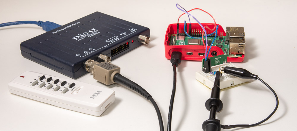
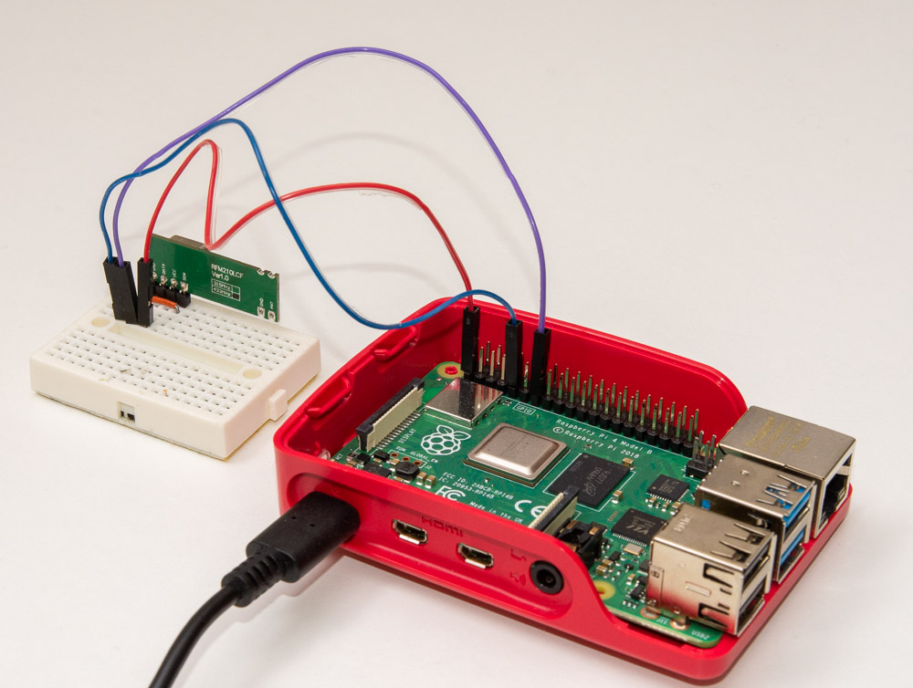
Raspberry Pi is nice also due to the fact that it has 3.3V voltage available on GPIO. Wiring up the 433 MHz receiver was a pretty elegant matter (again, there is a straight jumper connection between GND and last pin of the receiver):

1. Wire the receiver in
2. Start the script with python scan.py --raw (use -h option instead for help on command)
3. Press the Nexa remote button 1 during the 3 second recording interval

Here's how the output looks like (newline is added after delays longer than 5 ms):

36 1116 190 2805 55 14 43 2265 231 8216
57 87554
36 7409
76 4551 56 4281 95 2420 56 11327
13 4593 95 1056 76 692 13 53716
55 5990
14 37858
306 269 2592 248 288 250 1267 249 288 231 1287 248 288 231 1286 230 1286 250 268 250 1286 230 288 249 1269 248 288 249 1268 249 288 249 269 249 1307 229 269 249 1287 249 269 249 1288 229 288 249 1287 230 287 250 1268 249 287 231 1286 250 1267 249 288 249 269 249 1287 230 288 249 1288 248 269 249 1287 229 289 249 1269 248 288 230 1286 249 288 231 1287 229 288 250 1286 230 1287 230 307 230 288 230 1286 250 1268 248 307 230 1287 230 288 249 289 230 1286 249 269 249 1287 249 1268 248 289 230 288 249 1287 230 288 230 1286 250 287 230 1287 250 268 250 1267 249 10021
229 2630 230 288 250 1287 229 288 231 1286 249 269 249 1288 248 1267 249 288 230 1288 229 288 249 1267 250 288 249 1268 249 288 249 3867 248 249 288 1248 269 268 250 1267 250 268 250 1286 250 288 230 1286 249 1267 230 307 231 289 229 1287 249 288 230 1305 232 287 230 1305 230 289 230 1286 250 288 229 1287 249 269 250 1301 235 268 249 1286 231 1267 250 288 249 287 231 1286 250 1267 249 289 248 1287 230 288 249 288 231 1287 248 269 250 1286 230 1286 231 307 230 287 231 1286 249 288 231 1287 248 288 230 1287 230 288 230 1288 248 10002
248 2631 229 288 230 1286 261 277 230 1287 249 268 250 1286 231 1286 249 269 249 1287 230 288 250 1266 250 288 249 1267 249 290 248 269 249 1287 249 288 230 1287 249 268 250 1286 249 269 250 1287 229 288 250 1267 249 288 250 1268 248 1267 250 287 250 269 249 1288 229 287 250 1286 250 268 250 1287 229 288 250 1286 230 288 250 1268 248 269 249 1287 249 269 249 1288 248 1267 230 288 249 289 249 1268 248 1287 230 307 230 1268 268 269 249 288 231 1305 230 288 230 1287 249 1267 249 288 230 288 250 1288 227 288 230 1286 249 288 231 1289 248 288 230 1267 250 10021

Wow! It's actually pretty easy to spot the Nexa signals with 10 ms timeout between repeats! Note that this code is not differentiating which delay is logic HIGH and which is logic LOW, either you add initial measurement before starting edge detection (in which case there is small risk that the level will change before the detection is up...) or in the callback function, but I already knew which part of the signal is HIGH and which LOW so I did not bother this time.

Printing out the average edge lengths and "sequence string"

After spending the time in soundcard version to do smart clustering, I decided to use a bit simpler approach by measuring the average length of the signal portions. Just preset rough "centers" manually and assign the closest center to different signals. This makes average calculation much easier and does not require sklearn:

from collections import defaultdict

# Three timing buckets and their "character codes"
buckets = list(zip([250,1250,2500], 'x-_'))

lengths = defaultdict(list)
seq = []
for d in diff:
    if d < .7 * buckets[0][0] or d > 1.3 * buckets[-1][0]: # New
        print(f'{d} us ' if d < 1000 else f'\n{d/1000:.2f} ms\n', end='')
        if len(seq) > 10: # Print out longer sequences than 10 tokens
            print()
            for k in lengths:
                ls = sorted(lengths[k])
                print(f'{k}: avg {sum(ls) / len(ls):.2f} median {ls[len(ls)//2]}')
            print(''.join(seq))
        seq = []
        lengths = defaultdict(list)
    else:
        b = min((abs(d-a), c) for a,c in buckets)[1]
        seq.append(b) # add to letter sequence
        lengths[b].append(d) # save exact length

If you have not seen zip before, it basically combines two iterables into tuples, so buckets looks like this:

buckets = [(250, 'x'), (1250, '-'), (2500, '_')]

Signals shorter than 0.7x the shortest or longer than 1.3x the longest are displayed separately with actual timings (if section in the for loop, includes printing out completed sequences). Other values are grouped into their bucket and the actual length recorded in the else section. The output is rather easy to follow:

5.99 ms
14 us 
37.86 ms

10.02 ms

x: avg 256.64 median 249
_: avg 2592.00 median 2592
-: avg 1282.03 median 1286
xx_xxx-xxx-xxx-x-xxx-xxx-xxx-xxxxx-xxx-xxx-xxx-xxx-xxx-x-xxxxx-xxx-xxx-xxx-xxx-xxx-xxx-x-xxxxx-x-xxx-xxxxx-xxx-x-xxxxx-xxx-xxx-xxx-x

3.87 ms

x: avg 255.04 median 249
_: avg 2630.00 median 2630
-: avg 1278.71 median 1286
x_xxx-xxx-xxx-x-xxx-xxx-xxx-xxx

10.00 ms

x: avg 255.23 median 249
-: avg 1283.70 median 1286
xxx-xxx-xxx-xxx-x-xxxxx-xxx-xxx-xxx-xxx-xxx-xxx-x-xxxxx-x-xxx-xxxxx-xxx-x-xxxxx-xxx-xxx-xxx-x

10.02 ms

x: avg 256.15 median 250
_: avg 2631.00 median 2631
-: avg 1280.72 median 1286
x_xxx-xxx-xxx-x-xxx-xxx-xxx-xxxxx-xxx-xxx-xxx-xxx-xxx-x-xxxxx-xxx-xxx-xxx-xxx-xxx-xxx-x-xxxxx-x-xxx-xxxxx-xxx-x-xxxxx-xxx-xxx-xxx-x

10.02 ms

x: avg 256.73 median 250
_: avg 2631.00 median 2631
-: avg 1278.34 median 1286
x_xxx-xxx-xxx-x-xxx-xxx-xxx-xxxxx-xxx-xxx-xxx-xxx-xxx-x-xxxxx-xxx-xxx-xxx-xxx-xxx-xxx-x-xxxxx-x-xxx-xxxxx-xxx-x-xxxxx-xxx-xxx-xxx-x

410.21 ms

As short HIGH and LOW signals here produce the same "x", a high-low-high representing to spikes before a longer delay looks like xxx. So if you want to "count" the spikes, you can replace the xxxxx with 3, xxx with 2 and x with 1 to the a nicer looking representation. This is the first xx_xxx-xxx... signal:

11_2-2-2-1-2-2-2-3-2-2-2-2-2-1-3-2-2-2-2-2-2-1-3-1-2-3-2-1-3-2-2-2-1

Very nice! And all with less than 50 lines of code. You can find the full script here.

Sending the signal

After recovering the timings, doing the reverse of actually transmitting the signal is quite simple. I'm not covering this in detail, but you can use same wiring as for rpi-rf, connecting the 433 MHz transmitter to pin 17 on GPIO (it is between GND and pin 27 used in the receiving part) and copy-pasteing the signal. Note that I have added additional 'W' character to represent the 10 ms delay between repeats of the signal:

from RPi import GPIO
import time

wait = {'x': 256-50, '-': 1278-120, '_': 2630-120, 'W': 10000-50}
prg = "xx_xxx-xxx-xxx-x-xxx-xxx-xxx-xxxxx-xxx-xxx-xxx-xxx-xxx-x-xxxxx-xxx-xxx-xxx-xxx-xxx-xxx-x-xxxxx-x-xxx-xxxxx-xxx-x-xxxxx-xxx-xxx-x-xxx" \
    "Wx_xxx-xxx-xxx-x-xxx-xxx-xxx-xxxxx-xxx-xxx-xxx-xxx-xxx-x-xxxxx-xxx-xxx-xxx-xxx-xxx-xxx-x-xxxxx-x-xxx-xxxxx-xxx-x-xxxxx-xxx-xxx-x-xxx" \
    "Wx_xxx-xxx-xxx-x-xxx-xxx-xxx-xxxxx-xxx-xxx-xxx-xxx-xxx-x-xxxxx-xxx-xxx-xxx-xxx-xxx-xxx-x-xxxxx-x-xxx-xxxxx-xxx-x-xxxxx-xxx-xxx-x-xxx" \
    "Wx_xxx-xxx-xxx-x-xxx-xxx-xxx-xxxxx-xxx-xxx-xxx-xxx-xxx-x-xxxxx-xxx-xxx-xxx-xxx-xxx-xxx-x-xxxxx-x-xxx-xxxxx-xxx-x-xxxxx-xxx-xxx-x-xxx" \
    "Wx_xxx-xxx-xxx-x-xxx-xxx-xxx-xxxxx-xxx-xxx-xxx-xxx-xxx-x-xxxxx-xxx-xxx-xxx-xxx-xxx-xxx-x-xxxxx-x-xxx-xxxxx-xxx-x-xxxxx-xxx-xxx-x-xxx"
print(prg)

GPIO.setmode(GPIO.BCM)
GPIO.setup(17, GPIO.OUT)

for i,c in enumerate(prg):
    # set pin 17 high for 250 microseconds
    GPIO.output(17, GPIO.HIGH if (i&1) else GPIO.LOW)
    time.sleep((wait[c])/1e6)

# Clean up GPIO
GPIO.setup(17, GPIO.IN)
GPIO.cleanup()

The Gold Standard: Actual oscilloscope

All right! We have now looked at the RF receiver signal with Arduino, soundcard, and Raspberry Pi. Let's take a look!

I'm using my trusty PicoScope 2208B MSO with 128 million samples of memory, 2 channels with 100 MHz bandwidth and a multichannel logic analysis part. I'm using the analog measurement for this to view the signal.

Setting the resolution to 500 ms per grid unit and resolution to 1 million samples per second we get a really high resolution view of what is happening when the remote button is pressed twice:

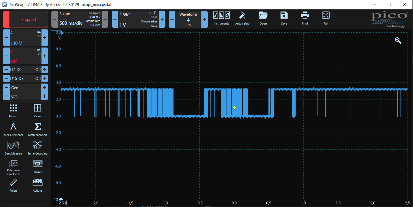
As the PicoScope is USB powered and RaspPi comes with its own power source which was 0.1V higher than PicoScope GND, I put a 1 kOhm resistor between the probe ground wire and the RaspPi GND. You can see a bit of fizz on the signal due to that.

Zooming in to the signal shows the familiar "spike" pattern — and the slight wobble introduced by the separete RaspPi power adapter, apologies for slightly unprofessional measuring setup. I recall PicoScope software can do differential measurements with two probes combined, but did not take advantage of such advanced features:

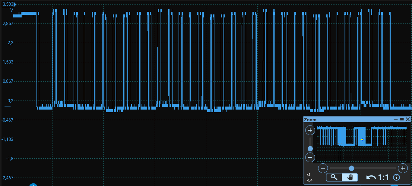
Now what about the resolution? Zooming in to the signal shows us in intimate detail the signal rising and falling:

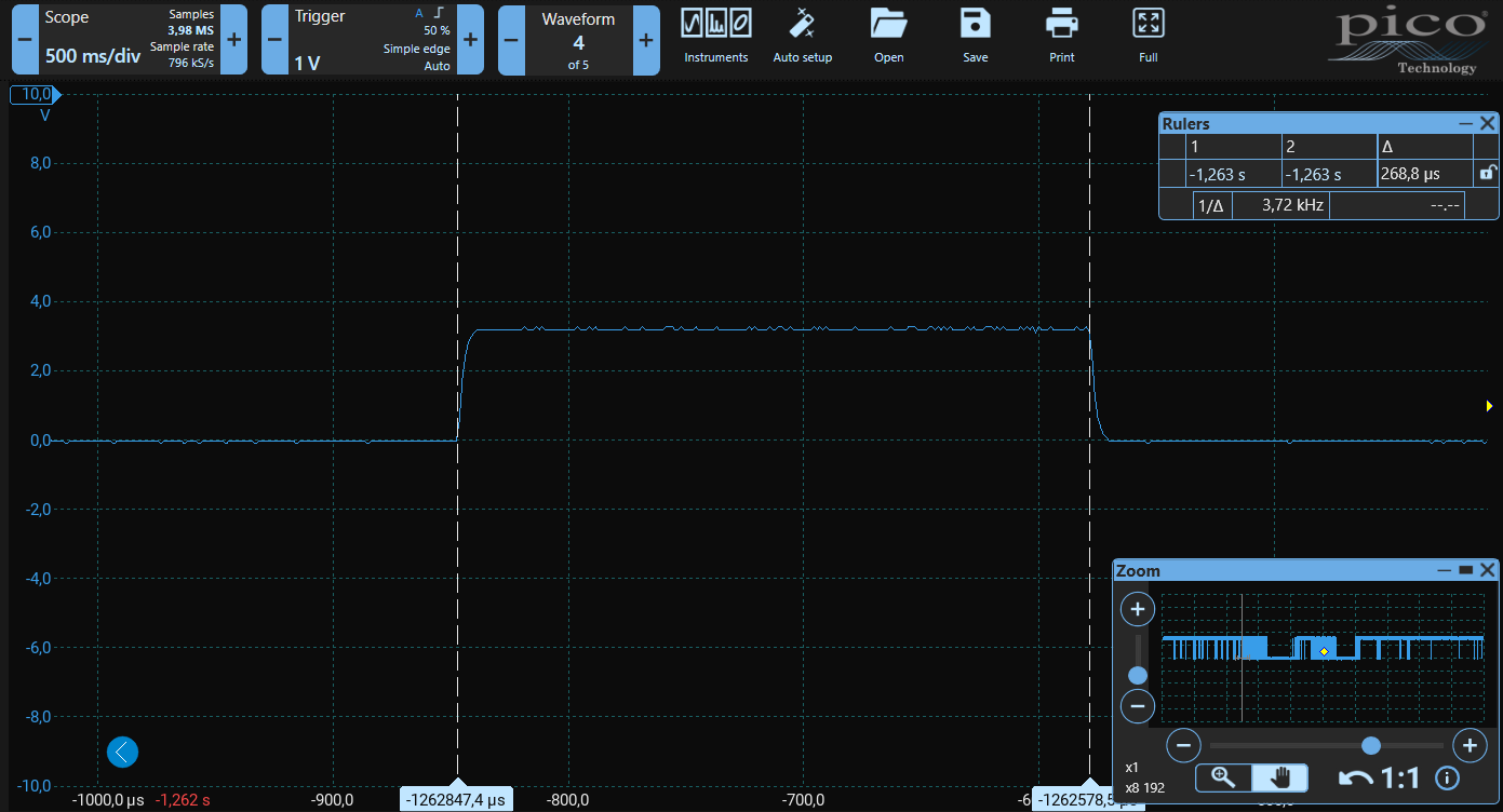
I've added rulers to measure the initial HIGH pulse width, about 268,8 microseconds. Now this is actually the exactly same signal I simultaneously recorded with the RaspPi. What did it store? 269 microseconds! Not bad! Let's look at the snippet and compare the first 8 pulses:

RaspPi	PicoScope	Level
306	306.8	LOW
269	268.4	HIGH
2592	2591	LOW
248	249.5	HIGH
288	287.4	LOW
250	250.2	HIGH
1267	1267	LOW
249	248.5	HIGH

I have to say that the RaspPi accuracy is quite remarkable. Obviously the Python implementation can react pretty much within a microsecond to the edge. With PicoScope the measurement is even more accurate, but for this frequency measurement (250 microseconds equals 40 kHz) the Pi is wholly adequate. I did not go through the whole sequence to see if there are occasional delays in the Pi measurements, but a few repeated measurements will fix that for this application.

Probably worth noting, that PicoScope is not breaking a sweat at this level, as 40 kHz is less than one thousandth of its 100 MHz maximum resolution. Benefits of using an actual oscilloscope, and especially a PC connected one is that the software is very powerful, there's easy zooming, measurements, and the PicoScope application can even measure edge widths etc. automatically, though you need to set up logic levels etc. before that.

Conclusion

Wow! What a journey. I've covered Arduino Uno, PC soundcard, Raspberry Pi 4 and PicoScope use for analyzing the radio signal from a 433 MHz smart power plug remote. Time for a quick summary:

	Arduino Uno	PC soundcard	Raspberry Pi 4	PicoScope
Benefits	Creap. Simple to program and wire, quite straightforward to view	Unlimited continuous measurement at 44/48 kHz	Accurate to microsecond level and virtually unlimited memory	Superior accuracy and bandwidth
Drawbacks	2 kB memory runs out almost immediately. Not very accurate without HW timer use	Additional resistors and wiring needed, separate power supply as well for RF receiver	Not an RTOS so may glitch every now and then	Overkill for this application, cost vs. alternatives

Note that for example RP2040 would pretty much combine the strengths of Arduino Uno and Raspberry Pi, with plentifiul memory for this application, and the real-time nature vs. Pi.

Now that we've covered the reverse engineering part, applying the learnings of sending the Nexa signals is an interesting next subject. I will likely return to thus later when I think of a fun project to apply that!