After a few busy weeks, I’ve finally arranged enough time to cover the details behind my color composite video decoding project I featured recently. Before you proceed, I suggest you read the previous post, as well as the one before that covers B/W decoding (this post builds on that one), and watch the video, if you haven’t already:

So, feel ready to learn about composite color coding, quadrature amplitude modulation (QAM)? Let’s get started! Before you get going, you can grab the example excel file so you can view the diagrams below in full size, and study the data and formulas yourself.

Combining luminance and color information

If we look at one line of video information (“scanline”), it’s basically a function of two things: luminance (brightness) and chrominance (color) information, combined to a single waveform/signal like this one I showed in my first article.

If we’d like to just have a black-and-white image, encoding it would be easy: Maximum voltage for white, minimum voltage for black, and the values between would simply be shades of grey. However, if we’d like to add color information to this signal, we need to get clever. What the engineers in the 1960’s did to get two things stuffed into one signal was to add color in sine wave modulated form on top of the luminance signal. With proper analog electronics, these two signals could then be separated from the receiving end.

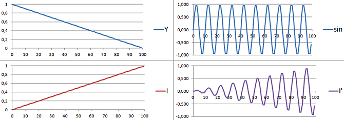
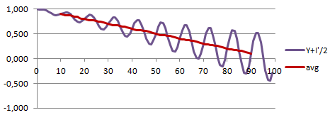
Using an example is the easiest way to explain what this “adding of signals” means, let’s take the example above. We have a line with brightness going from one to zero (Y), and “color” from zero to one (I). To modulate the color (I) signal with a sine wave, we simply multiply I with the wave, and get I’ as a result. Notice how the amplitude of the modulated signal (I’) changes with I, not the position. So if you’d take an average of I’ over 1 wavelength (or any multiple of it), you’d get about zero – not exactly zero unless I is constant, but close enough as we’ll see later. Adding Y and I’ together, we have the combined “brightness plus color information” signal:

To keep I’ from dominating the signal, I divided it by 2 – similar scaling is done with real video signal. As we can see, the average of the signal correlates with Y, and the amplitude of sine wave with I – excellent! But how to extract this information in the other end? In analog world, we’d use an oscillator synced to the sine wave (that is why there is a sine wave called “color burst” in every line before the actual data), but in digital world we can’t rely on properties of physical components, but have to rely on maths instead.

Let’s assume for a while that our sine wave carrier frequency is much higher than the frequency content of both luminance and chroma information – i.e. over a single sine wave period, both Y and I stay rather constant (for example, while sine wave goes all the way from zero to one, zero, minus one and back to zero again, Y and I both change less than 0.01). So for a single period, the signal is essentially:

S(x) = Y + I / 2 * sin(x)

Where x goes from 0 to 2*Pi. From the above formulation, it’s obvious that if we calculate the average of S over the period, we get “Y” (remember that the average of a sine wave is zero, because positive and negative values cancel out). But how to get “I”? Simple, let’s multiply it by the carrier wave again, sin(x):

S(x)*sin(x) = Y * sin(x) + I/2 * sin^2(x)

If we use the trigonometric identity sin^2(x) = 1/2 – 1/2 * cos(2x), we get:

S(x)*sin(x) = Y * sin(x) + I/4 – I/4 * cos(2x)

It’s again easy to see (integrate from 0 to 2*Pi if you’re not confident) that the average of S*sin over one period is I/4. So we just need to multiply the signal with the original sine wave, take the average and multiply it by 4 to get “I”! It turns out, that not only does this work in practice, it also works quite well even if Y and I are not constant! Below you can see the multiplied S*sin signal (“mul”) and running average of 20 consecutive values (2 sine wave periods) – notice how we “extracted” I from the composite signal!

As you can see, the “extracted” I is not exactly the original I, because our “running average” method is not an optimal low-pass filter. However, in practice it good enough (and a lot better than standard discrete low pass filter, trust me, I tried).

Adding a second color channel

So now that we can add two signals into one and separate them again, you’d think we would be done. Not so fast! To get full color, we actually need three components: red, green, and blue. So even if we transform these three values to luminance and chroma, we still need two components for color!

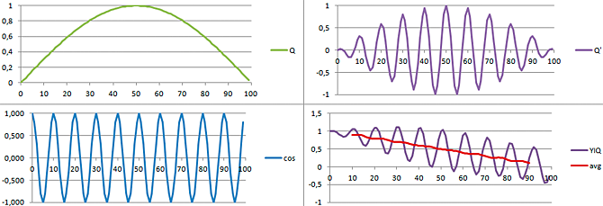
Thankfully, the sine wave modulation described above has an additional benefit: We can actually modulate the second color signal (Q) with cos(x), and it will cancel itself out in the calculations above when we multiply the signal by sin(x). And when we multiply with cos(x) instead, the sin(x) terms (I) cancel out! How amazing is that? Not very amazing, if you have studied Fourier transformations and know that sin(x) and cos(x) are orthogonal (I have, but that was ten years ago :), but for most people, I’d say it is pretty mind-blowing.

Below, you can see our second color signal “Q”, its carrier wave “cos”, the resulting modulated signal “Q'”, and the YIQ signal which has luminance and both chroma signal combined (the full formula is YIQ = Y + I/2*sin(x) + Q/2*cos(x)):

The nature of the sine and cosine wave is such, that adding two of them together actually creates a wave, where the exact amplitude and phase at a given point is determined by the two original waves. The math doesn’t change, but if you don’t look carefully, it looks like we just lost the first color signal, “I”. To prove it’s not so, here are the sin(x) and cos(x) multiplied signals, and their running averages, showing that the YIQ signal really does contain both chroma components (I is on left, Q on right):

Color space conversion

With the techniques presented above (averaging, multiplying with sine and cosine carrier waves), we can extract the brightness and color information from the NTSC signal. What remains is the conversion of these Y, I, Q values to RGB (red, green, blue). This is done with simple multiplication, and is explained nicely in Wikipedia:

http://en.wikipedia.org/wiki/YIQ

If you have trouble understanding the matrix representation of YIQ color space, you can start with a simpler model. Let’s assume we’d like to convert a R, G, B value to “brightness, red, green” (brg) color space. We’d use the following formulas:

b = (R + G + B) / 3 = 0.333 * R + 0.333 * G + 0.333 * B r = R = 1.000 * R + 0.000 * G + 0.000 * B g = G = 0.000 * R + 1.000 * G + 0.000 * B

As a matrix, this would be represented as:

| 0.333 0.333 0.333 | | 1.000 0.000 0.000 | = M | 0.000 1.000 0.000 |

So a matrix is essentially just a shorthand for multipliers used in color conversion. Calculating brg value from RGB vector is done thus:

| 0.333 0.333 0.333 | | R | | 0.333 * R + 0.333 * G + 0.333 * B | | 1.000 0.000 0.000 | x | G | = | 1.000 * R + 0.000 * G + 0.000 * B | | 0.000 1.000 0.000 | | B | | 0.000 * R + 1.000 * G + 0.000 * B |

| (R+G+B) * .333 | = | R | | G |

Now if we have a Brg value, how do we get RGB? Easily:

R = r
G = g
B = 3*b – r – g

Again, this can be represented as a matrix (you can use the matrix multiplication example above to verify you actually get the correct formulas):

| 0.000 1.000 0.000 | | b | | R | | 0.000 0.000 1.000 | x | r | = | G | | 3.000 -1.000 -1.000 | | g | = | B |

Once you’ve wrapped your head around how these work, you shouldn’t have any problems understanding the YIQ to RGB conversion. Another common color space is YUV, and it turned out my Raspberry Pi actually used one variant of that. When you look through the internet, you’ll find that there are several slightly different component weights (conversion matrices) for YUV and YIQ, so you might need to try out a few until you find the one your source is actually using!

Conclusions

In this post, I covered the quadrature amplitude modulation (QAM) used in NTSC composite signal encoding, as well as short introduction to color space conversions. Armed with these, we can convert a composite signal in YIQ or YUV color space to a RGB component signal.

The article is getting quite long, so I think I’ll write another post later on implementation details of these techniques in code level. There are also some issues not covered in here that arise when implementing the conversion, such as syncing to scanline color carrier phase, and (auto-)detecting color signal amplitudes from the NTSC signal. So stay tuned for a follow-up!